Sheafification Functor and Arbitrary Monetary Value Measure. Part 3

Here are Part 1 and Part 2

Let A be a fixed set of axioms. Then for a given arbitrary monetary value measure Ψ can we make a good alternative for it? In other words, can we find a monetary value measure that satisfies A and is the best approximation of the original Ψ? For a Grothendieck topology J on χ, define Sh(χ, J) ⊂ Set^χop to be a full sub-category whose objects are all sheaves for J. Then, it is well known that ∃ a left adjoint π_J in the following diagram.

Sh(χ, J) → Set^χop

Sh(χ, J) ←_πJ Set^χop

π_J (Ψ) ← Ψ

The functor π_J is known as Sheafification functor, which has the following limit cone:

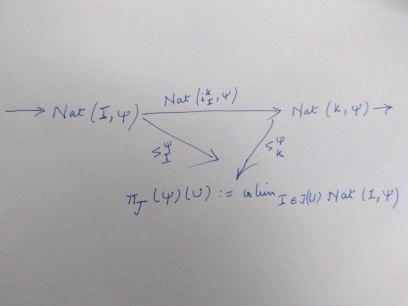
for sieves I, K and U. This also satisfies the following theorem.

1.0 If π_J (Ψ) is a sheaf for J

1.1 If Ψ is a sheaf for J, then for any U ∈ χ,  π_J (Ψ)(U) ≅ L(U)

The theorem suggests that for an arbitrary monetary value measure, the sheafification functor provides one of its closest monetary value measures that may satisfy the given set of axioms. To make this certain, we need a following definition.

2.0 Let A be a set of axioms of monetary value measures

2.1 M(A) := the collection of all monetary value measures satisfying A

2.2 M_O := collection of all monetary value measures

2.3 A is called complete if

π_JM(A) (M_O) ⊂ M(A)

3.0 Let A be a complete set of axioms. Then, for a monetary value measure Ψ ∈ M_O, π_JM(A(Ψ) is the monetary value measure that is the best approximation satisfying A.

Let us investigate if the set of axioms of concave monetary value measures is complete in the case of Ω = {1, 2, 3} with a σ-field F := 2^Ω

We enumerate all possible sub-σ-fields of Ω, that is, the shape of the category χ = χ(Ω),

where,

U_∞ := F := 2^Ω

U₁ := {Φ, {1}, {2, 3}, Ω}

U₂ := {Φ, {2}, {1, 3}, Ω}

U₃ := {Φ, {3}, {1, 2}, Ω}

U₄ := {Φ, Ω}

The Banach spaces defined by the elements of χ are

L_∞ := L := L(U_∞) := {a, b, c | a, b, c ∈ ℜ}

L₁ := L(U₁) := {a, b, b | a, b ∈ ℜ}

L₂ := L(U₂) := {a, b, a | a, b ∈ ℜ}

L₃ := L(U₃) := {a, a, c | a, c ∈ ℜ}

L₀ := L(U₀) := {a, a, a, | a ∈ ℜ}

Then a monetary value measure Ψ : χ^op → Set on χ is determined by the following six functions

We will investigate its concrete shape one by one by considering axioms it satisfies.

For Ψ¹_∞ : L_∞ → L₁, we have by the cash invariance axiom,

Ψ¹_∞ (a, b, c) = Ψ¹_∞ ((0, b – c, 0) + (a, c, c))

= Ψ¹_∞ ((0, b – c, 0)) + (a, c, c)

= (f₁₂ (b – c), f₁₁ (b – c), f₁₁ (b – c)) + (a, c, c)

= (f₁₂ (b – c) + a, f₁₁ (b – c) + c, f₁₁ (b – c)+ c)

where f₁₁, f₁₂ : ℜ → ℜ are defined by (f₁₂(x), f₁₁(x), f₁₁(x)) = Ψ¹_∞ (0, x, 0).

Similarly, if we define nine functions

f₁₁, f₁₂, f₂₁, f₂₂, f₃₁, f₃₂, g₁, g₂, g₃ : ℜ → ℜ by

(f₁₂(x), f₁₁(x), f₁₁(x)) = Ψ¹_∞(0, x, 0)

(f₂₁(x), f₂₂(x), f₂₁(x)) = Ψ²_∞(0, 0, x)

(f₃₁(x), f₃₁(x), f₃₂(x)) = Ψ³_∞(x, 0, 0)

(g₁(x), g₁(x), g₁(x)) = Ψ⁰₁(x, 0, 0)

(g₂(x), g₂(x), g₂(x)) = Ψ⁰₂(0, x, 0)

(g₃(x), g₃(x), g₃(x)) = Ψ⁰₃(0, 0, x)

We can represent the original six functions by nine functions

Ψ¹_∞(a, b, c) = (f₁₂(b – c) + a, f₁₁(b – c) + c, f₁₁(b – c) + c),

Ψ²_∞(a, b, c) = (f₂₁(c – a) + a, f₂₂(c – a) + a, f₂₁(c – a) + a),

Ψ³_∞(a, b, c) = (f₃₁(a – b) + b, f₃₁(a – b) + b, f₃₂(a – b) + c),

Ψ⁰₁(a, b, b) = (g₁(a – b) + b, g₁(a – b) + b, g₁(a – b) + b),

Ψ⁰₂(a, b, a) = (g₂(b – a) + a, g₂(b – a) + a, g₂(b – a) + a),

Ψ⁰₃(a, a, c) = (g₃(c – a) + a, g₃(c – a) + a, g₃(c – a) + a)

Next by the normahzation axiom, we have

f₁₁(0) = f₁₂(0) = f₂₁(0) = f₂₂(0) = f₃₁(0) = f₃₂(0) = g₁(0) = g₂(0) = g₃(0) = 0

partially differentiating the function in Ψ¹_∞(a, b, c), we have

∂Ψ¹_∞(a, b, c)/∂a = (1, 0, 0)

∂Ψ¹_∞(a, b, c)/∂b = (f’₁₂(b – c), f’₁₁(b – c), f’₁₁(b – c))

∂Ψ¹_∞(a, b, c)/∂c = (- f’₁₂(b – c), 1 –  f’₁₁(b – c), 1 –  f’₁₁(b – c))

Therefore, by the monotonicity, we have f’₁₂(x) = 0 and 0 ≤ f’₁₁ ≤ 1. Then by the result of the normalization axiom, we have

x ∈ ℜ, f₁₂(x) = 0. Hence, ∀ x ∈ ℜ,

f₁₂(x) = f₂₂(x) = f₃₂(x) = 0

With this knowledge, let us redefine the three functions f₁, f₂, f₃ : ℜ → ℜ by

(0, f₁(x), f₁(x)) = Ψ¹_∞(0, x, 0)

(f₂(x), 0, f₂(x)) = Ψ²_∞(0, 0, x)

(f₃(x), f₃(x), 0) = Ψ³_∞(x, 0, 0)

Then, we have a new representation of the original six functions

Ψ¹_∞(a, b, c) = (a, f₁(b – c) + c, f₁(b – c) + c)

Ψ²_∞(a, b, c) = (f₂(c – a) + a, b, f₂(c – a) + a)

Ψ³_∞(a, b, c) = (f₃(a – b) + b, f₃(a – b) + b, c)

Ψ⁰₁(a, b, b) = (g₁(a – b) + b, g₁(a – b) + b, g₁(a – b) + b)

Ψ⁰₂(a, b, a) = (g₂(b – a) + a, g₂(b – a) + a, g₂(b – a) + a)

Ψ⁰₃(a, a, c) = (g₃(c – a) + a, g₃(c – a) + a, g₃(c – a) + a)

Thinking about the composition rule, we have

Ψ⁰_∞ = Ψ⁰₁ o Ψ¹_∞ = Ψ⁰₂ o Ψ²_∞ = Ψ⁰₃ o Ψ³_∞

g₁(a – f₁(b – c) – c) + f₁(b – c) + c

= g₂(b – f₂(c – a) – a) + f₂(c – a) + a

=g₃(c – f₃(a – b) – b) + f₃(a – b) + b

………..

 

Advertisement